Even though weather stations are capable to record a huge amount of data, there is also a lot of work to do to obtain some information. For example, if observations are taken every hour, you’ll have 8700 records in 1 year!

So, in this post we’re going to:

• Write functions in R to aggregate the big amount of information provided by weather stations.
• Make these functions as general as possible in terms of the structure of the input data (time series data) in order to simplify downstream analysis of this data.
• Finally, we’re going to plot our results to reach some conclusions about the weather in one town in San Luis Province, Argentina.

    We chose to work with data from La Calera. Take a look to our target site on the map! It’s a little town in the Northwest of the San Luis Province, located in a semiarid region. It makes this town and its neighbors really interesting places to work with because in this desert places, climate has well defined seasons and rainfalls occurs mainly in a few months of the year.

    We have already downloaded the .csv file of La Calera from the REM website, and you can find it here . Ok! Let’s work!

Tidying data – Writing an R function

    First, we’re going to read the .csv with R and see its structure. How many rows does it have? Which are the first and the last dates? Which are the variables recorded? We’ll use head(), nrow() and str() to see it.

    As you can see, this weather station recorded rainfalls (mm), humidity (%) and temperature (°C) every hour. Data recording started on October 2007 and finished on April 2018 (the day that we downloaded the .csv). There are in total more than 91.000 observations for each variable!. Hourly data won’t allow us to find some of the climatic patterns that we are looking for, so, we need to summarize its information first as daily data and then as monthly data.

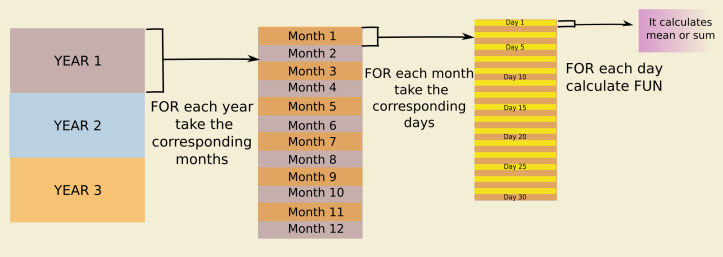
   We’re going to start writing an R function that will be useful for organize data in different stages of the analysis (see the flowchart below) . It takes the date of every row and splits it up in 3 columns: one column with the day’s number, a second column with the month’s number, and the last one with the year. In this function, we’re going to use the lubridate package. This package has some useful functions that we need: day(), month() and year() which extract the corresponding time component from a given date. In the following functions, we’ll use these new columns to subset the data.

If we use our function, we get:

Aggregate daily data – Writing an R function

    Now, we’re going to aggregate our hourly data in daily data. We wrote another function that uses the columns that we have obtained to subset the data. For each day,  we created a subset with its corresponding hours and calculated the daily mean or the sum for data (see the diagram below).

 As we’re working with meteorological data, the sum will be useful for precipitations, and the mean for temperature. We calculated the daily mean value as an average of extreme hourly values, due to daily mean temperature it’s commonly estimated as the average of minimum and maximum temperatures (see http://climod.nrcc.cornell.edu/static/glossary.html and Dall’Amico and Hornsteiner, 2006).  This is:

For each day of hourly data we have the following set:  so we calculate the average as:

In R, we can do it using max() and min() functions. But wait! It’s normal that weather stations don’t work during some days, so you can have entire days where they only recorded “NAs”. So, you have to keep this in mind, because max() and min() functions will return you:

    To avoid that, we used an if…else statement in  line 32.

Exploratory plots – Daily data from La Calera

Let’s plot daily data to look for patterns!

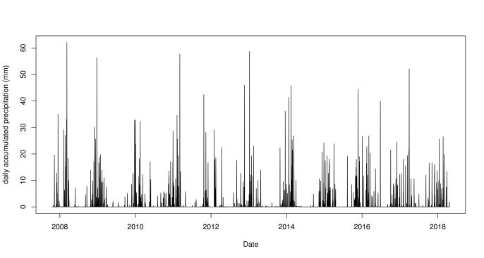
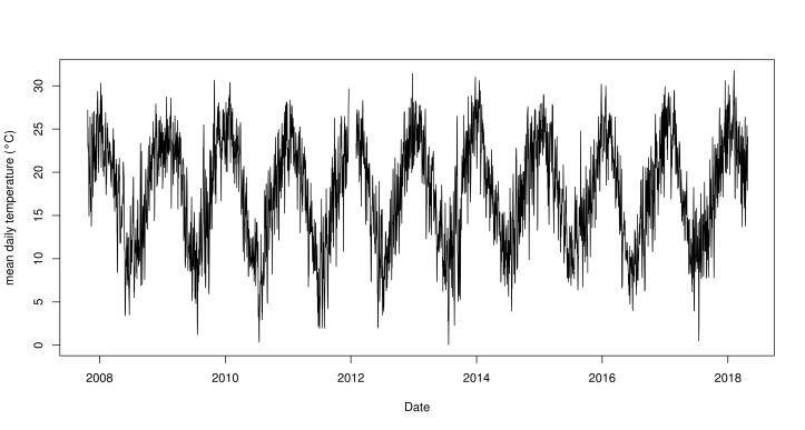
We’ve already have our first results! Rainfalls are higher during a period of each year, and between periods there are gaps of dry weather. On the other side, mean temperatures have an oscillating pattern, reaching 30°C in summer and 0°C in winter. So, as we expected from this temperate desert place, seasons are well-defined and temperature have a wide range through the year.

Aggregate monthly data – Writing an R function

  Ok, let’s continue a bit more! To aggregate from daily data to monthly data, we have to use again the first function (add the time component’s columns) and then build a function with “for loops” similar to the second function. In this case, we didn’t use max() or min() functions, because monthly means are simply the average of daily means per month.

    We ran the function:

and we obtained the followings monthly time series:

Exploratory plots – Monthly data from La Calera

    To end this analysis, we’re going to do an exploratory analysis of our monthly data. For this we are going to make a multiple barplot using a ‘for loop’ and an overlayed lineplot for each one of the years in the dataset.

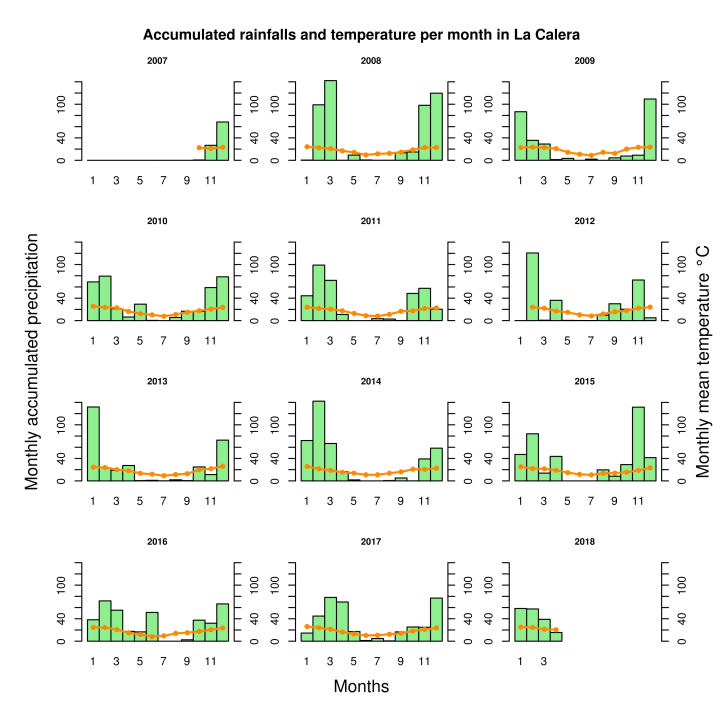
    As we previously saw, rains are concentrated only in some months. We can distinguish from the bar charts that La Calera has a dry period during winter, when temperatures are lower, and a rainy period during the warm seasons.

    Well, the analysis about yearly means of accumulated precipitations and temperatures  it is now up to you!

   You can see the entire R script of this post in here, and remember that all of our scripts and data used for the blog are available in our GitHubs.

    And, if you’re interested in other analysis of different kinds of time series data, you could take a look to our other post:

• Exchange rate (ARS / USD) – Part I – Getting data – AWK and R
• Exchange rate (ARS / USD) – Part II – Writing R functions to analyze simple variations and making animations to visualize them

轉貼自： Monkeysworking